2.2.2. Parsl: Molecular design ML-in-the-loop workflow

This notebook demonstrates a simple molecular design application where we use machine learning to guide which computations we perform. The objective of this application is to identify which molecules have the largest ionization energies (IE, the amount of energy required to remove an electron).

IE can be computed using various simulation packages (here we use xTB ); however, execution of these simulations is expensive, and thus, given a finite compute budget, we must carefully select which molecules to explore. We use machine learning to predict high IE molecules based on previous computations (a process often called active learning). We iteratively retrain the machine learning model to improve the accuract of predictions. The resulting ML-in-the-loop workflow proceeds as follows.

In this notebook, we use Parsl to execute functions (simulation, model training, and inference) in parallel. Parsl allows us to establish dependencies in the workflow and to execute the workflow on arbitrary computing infrastructure, from laptops to supercomputers. We show how Parsl’s integration with Python’s native concurrency library (i.e., `concurrent.futures <https://docs.python.org/3/library/concurrent.futures.html#module-concurrent.futures>`__) let you write applications that dynamically respond to the completion of asynchronous tasks.

%cd /tutorials/molecular-design-parsl-demo
%matplotlib inline

from matplotlib import pyplot as plt
from chemfunctions import compute_vertical
from concurrent.futures import as_completed
from tqdm.notebook import tqdm
from parsl.executors import HighThroughputExecutor
from parsl.app.python import PythonApp
from parsl.app.app import python_app
from parsl.config import Config
from time import monotonic
import parsl
import pandas as pd
import numpy as np

2.2.2.1. Define problem

We first define configuration parameters for the app, specifically the search space of molecules (selected randomly from the QM9 database) and parameters controlling the optimization algorithm (the number of initial simulations, total moleucles to be evaluated, and the number of molecules to be evaluated in a batch).

search_space = pd.read_csv('data/QM9-search.tsv', delim_whitespace=True).sample(1024)  # Our search space of molecules

initial_count: int = 8  # Number of calculations to run at first

search_count: int = 16   # Number of molecules to evaluate in total

batch_size: int = 4  # Number of molecules to evaluate in each batch of simulations

2.2.2.2. Set up Parsl

We now configure Parsl to make use of available resources. In this case we configure Parsl to run on the local machine with two workers. One of the benefits of Parsl is that we can change this configuration to make use of different resources without modifying the following workflow. For example, we can configure Parsl to use more cores on the local machine or to use many nodes on a Supercomputer or Cloud. The Parsl website describes how Parsl can be configured for different resources.

config = Config(
    executors=[HighThroughputExecutor(
        max_workers=2, # Allows a maximum of two workers
    )]
)

parsl.load(config)

<parsl.dataflow.dflow.DataFlowKernel at 0x7fb10d7d7ac0>

2.2.2.3. Make an initial dataset

We need data to train our ML models. We’ll do that by selecting a set of molecules at random from our search space, performing some simulations on those molecules, and training on the results.

In `chemfunctions.py <./chemfunctions.py>`__, we have defined a function compute_vertical that computes the “vertical ionization energy” of a molecule (a measure of how much energy it takes to strip an electron off the molecule). compute_vertical takes a string representation of a molecule in SMILES format as input and returns the ionization energy as a float. Under the hood, it is running xTB to perform a series of quantum chemistry computations.

2.2.2.3.1. Execute a first simulation

We need to prepare this function to run with Parsl. All we need to do is wrap this function with Parsl’s python_app:

compute_vertical_app = python_app(compute_vertical)
compute_vertical_app

<parsl.app.python.PythonApp at 0x7fb0ae128970>

This new object is a Parsl PythonApp. It can be invoked like the original function, but instead of immediately executing, the function may be run asynchronously by Parsl. Instead of the result, the call will immediately return a Future which we can use to retrieve the result or obtain the status of the running task.

For example, invoking the compute_verticle_app with the SMILES for water, O, returns a Future and schedules compute_verticle for execution in the background.

future = compute_vertical_app('O') #  Run water as a demonstration (O is the SMILES for water)
future

<AppFuture at 0x7fb0ae128820 state=pending>

We can access the result of this computation by asking the future for the result(). If the computation isn’t finished yet, then the call to .result() will block until the result is ready.

ie = future.result()
print(f"The ionization energy of {future.task_def['args'][0]} is {ie:.2f} Ha")

The ionization energy of O is 0.67 Ha

2.2.2.3.2. Scale the simulation

It is trivial now to scale our simulation and run it for several different molecules and gather their results.

We use a standard Python loop to submit a set of simulations for execution. As above, each invocation returns a Future immediately, so this code should finish within a few milliseconds.

Because we never call .result(), this code does not wait for any results to be ready. Instead, Parsl is running the computations in the background. Parsl manages sending work to each worker process, collecting results, and feeding new work to workers as new tasks are submitted.

%%time
smiles = search_space.sample(initial_count)['smiles']
futures = [compute_vertical_app(s) for s in smiles]
print(f'Submitted {len(futures)} calculations to start with')

Submitted 8 calculations to start with
CPU times: user 13.1 ms, sys: 10.8 ms, total: 23.9 ms
Wall time: 21 ms

The futures produced by Parsl are based on Python’s native “Future” object, so we can use Python’s utility functions to work with them.

As an example, we can build a loop that submits new computations if previous ones fail. This happens not too infrequently with our simulation application.

We use as_completed to take an iterable (in this case a list) of futures and to yeild as each future completes. Thus, we progress and handle each simulation as it completes

We also use, Future.exception() rather than the similar Future.result(). Future.exception() behaves similarly in that it will block until the relevant task is completed, but rather than return the result, it returns any exception that was raised during execution (or None if not). In this case, if the future returns an exception we simply pick a new molecule and re-execute the simulation.

train_data = []
while len(futures) > 0:
    # First, get the next completed computation from the list
    future = next(as_completed(futures))

    # Remove it from the list of still-running tasks
    futures.remove(future)

    # Get the input
    smiles = future.task_def['args'][0]

    # Check if the run completed successfully
    if future.exception() is not None:
        # If it failed, pick a new SMILES string at random and submit it
        print(f'Computation for {smiles} failed, submitting a replacement computation')
        smiles = search_space.sample(1).iloc[0]['smiles'] # pick one molecule
        new_future = compute_vertical_app(smiles) # launch a simulation in Parsl
        futures.append(new_future) # store the Future so we can keep track of it
    else:
        # If it succeeded, store the result
        print(f'Computation for {smiles} succeeded')
        train_data.append({
            'smiles': smiles,
            'ie': future.result(),
            'batch': 0,
            'time': monotonic()
        })

Computation for CC12COC1(C)C1OC21 failed, submitting a replacement computation
Computation for OC12CCC1NC2C#N failed, submitting a replacement computation
Computation for CC12C3N4CC(C14)C23O failed, submitting a replacement computation
Computation for O=C1CCC1NCC#N succeeded
Computation for NC(=O)NCC#CCO succeeded
Computation for CCC1CC2OC12 succeeded
Computation for CC1(C)OC(=N)C1(C)C succeeded
Computation for C1C2CC3=CCOC1C23 failed, submitting a replacement computation
Computation for C1CC2(CCOC2)CO1 succeeded
Computation for CN1CC(N=C1)C#N succeeded
Computation for O=C1CC2CCC3C2C13 succeeded
Computation for O=C1NC2CC11CCC21 failed, submitting a replacement computation
Computation for O=CC1=CC2CCC1C2 succeeded

We now have an initial set of training data. We load this training data into a pandas DataFrame containing the randomly samples molecules alongside the simulated ionization energy (ie). In addition, the code above has stored some metadata (batch and time) which we will use later.

train_data = pd.DataFrame(train_data)
train_data

	smiles	ie	batch	time
0	O=C1CCC1NCC#N	0.492704	0	26421.812311
1	NC(=O)NCC#CCO	0.492472	0	26440.254361
2	CCC1CC2OC12	0.514080	0	26464.257546
3	CC1(C)OC(=N)C1(C)C	0.504155	0	26498.323339
4	C1CC2(CCOC2)CO1	0.491403	0	26522.577064
5	CN1CC(N=C1)C#N	0.487846	0	26548.199886
6	O=C1CC2CCC3C2C13	0.499828	0	26556.459605
7	O=CC1=CC2CCC1C2	0.503186	0	26580.873453

2.2.2.4. Train a machine learning model to screen candidate molecules

Our next step is to create a machine learning model to estimate the outcome of new computations (i.e., ionization energy) and use it to rapidly scan the search space.

To start, let’s make a function that uses our prior simulations to train a model. We are going to use RDKit and scikit-learn to train a nearest-neighbor model that uses Morgan fingerprints to define similarity (see notes from a UChicago AI course for more detail). In short, the function trains a model that first populates a list of certain substructures (Morgan fingerprints, specifically) and then trains a model which predicts the IE of a new molecule by averaging those with the most similar substructures.

We want to use Parsl here to scale the model and to later combine it into our ML-in-the-loop workflow. To do so, we define the function using python_app. This time, python_app is used as a decorator directly on the function definition (earlier we defined a regular function, and then applied python_app afterwards).

@python_app
def train_model(train_data):
    """Train a machine learning model using Morgan Fingerprints.

    Args:
        train_data: Dataframe with a 'smiles' and 'ie' column
            that contains molecule structure and property, respectfully.
    Returns:
        A trained model
    """
    # Imports for python functions run remotely must be defined inside the function
    from chemfunctions import MorganFingerprintTransformer
    from sklearn.neighbors import KNeighborsRegressor
    from sklearn.pipeline import Pipeline


    model = Pipeline([
        ('fingerprint', MorganFingerprintTransformer()),
        ('knn', KNeighborsRegressor(n_neighbors=4, weights='distance', metric='jaccard', n_jobs=-1))  # n_jobs = -1 lets the model run all available processors
    ])

    return model.fit(train_data['smiles'], train_data['ie'])

Now let’s execute the function and run it asynchronously with Parsl

train_future = train_model(train_data)

One of the unique features of Parsl is that it can create workflows on-the-fly directly from Python. Parsl workflows are chains of functions, connected by dynamic depencies (i.e., data passed between Parsl apps), that can run in parallel when possible.

To establish the workflow, we pass the future created by executing one function an input to another Parsl function.

As an example, let’s create a function that uses the trained model to run inference on a large set of molecules and then another that takes many predictions and concatenates them into a single collection. The sequential workflow is implemented as follows.

train_model --> run_model --> combine_inferences

@python_app
def run_model(model, smiles):
    """Run a model on a list of smiles strings

    Args:
        model: Trained model that takes SMILES strings as inputs
        smiles: List of molecules to evaluate
    Returns:
        A dataframe with the molecules and their predicted outputs
    """
    import pandas as pd
    pred_y = model.predict(smiles)
    return pd.DataFrame({'smiles': smiles, 'ie': pred_y})

@python_app
def combine_inferences(inputs=[]):
    """Concatenate a series of inferences into a single DataFrame
    Args:
        inputs: a list of the component DataFrames
    Returns:
        A single DataFrame containing the same inferences
    """
    import pandas as pd
    return pd.concat(inputs, ignore_index=True)

Now we’ve created our Parsl apps, we can chop up the search space into chunks, and invoke run_model once for each chunk of the search space.

Note: we pass train_future (the future created from the training function above) as input to run_model. Parsl will wait for the training to be complete (i.e., the future to be resolved) before executing run_model.

# Chunk the search space into smaller pieces, so that each can run in parallel
chunks = np.array_split(search_space['smiles'], 64)
inference_futures = [run_model(train_future, chunk) for chunk in chunks]

While we are running inferences in parallel we can define the final part of the workflow to combine results into a single DataFrame using combine_inferences.

We pass the inference_futures as inputs to combine_inferences such that Parsl knows to establish a dependency between these two functions. That is, Parsl will ensure that train_future must complete before any of the run_model tasks start; and all of the run_model tasks must be finished before combine_inferences starts.

# We pass the inputs explicitly as a named argument "inputs" for Parsl to recognize this as a "reduce" step
#  See: https://parsl.readthedocs.io/en/stable/userguide/workflow.html#mapreduce
predictions = combine_inferences(inputs=inference_futures).result()

After completing the inference process we now have predicted IE values for all molecules in our search space. We can print out the best five molecules, according to the trained model:

predictions.sort_values('ie', ascending=False).head(5)

	smiles	ie
174	CCC1CC2OC12	0.514080
184	OCCC1CC(CO)O1	0.505487
372	NC1COC2=C1ON=C2	0.505344
167	CC12C3N1CC2OC3=O	0.505340
160	CC(C=O)C1C(C)C1C	0.505315

We have now created a Parsl workflow that is able to train a model and use it to identify molecules that are likely to be good next choices for simulations. Time to build a model-in-the-loop workflow.

2.2.2.5. Model-in-the-Loop Workflow

We are going to build an application that uses a machine learning model to pick a batch of simulations, runs the simulations in parallel, and then uses the data to retrain the model before repeating the loop.

Our application uses train_model, run_model, and combine_inferences as above, but after running an iteration it picks the predicted best molecules and runs the compute_vertical_app to run the xTB simulation. The workflow then repeatedly retrains the model using these results until a fixed number of molecule simulations have been trained.

with tqdm(total=search_count) as prog_bar: # setup a graphical progress bar
    prog_bar.update(len(train_data))
    batch = 1
    already_ran = set(train_data['smiles'])
    while len(train_data) < search_count:

        # Train and predict as show in the previous section.
        train_future = train_model(train_data)
        inference_futures = [run_model(train_future, chunk) for chunk in np.array_split(search_space['smiles'], 64)]
        predictions = combine_inferences(inputs=inference_futures).result()

        # Sort the predictions in descending order, and submit new molecules from them
        predictions.sort_values('ie', ascending=False, inplace=True)
        sim_futures = []
        for smiles in predictions['smiles']:
            if smiles not in already_ran:
                sim_futures.append(compute_vertical_app(smiles))
                already_ran.add(smiles)
                if len(sim_futures) >= batch_size:
                    break

        # Wait for every task in the current batch to complete, and store successful results
        new_results = []
        for future in as_completed(sim_futures):
            if future.exception() is None:
                prog_bar.update(1)
                new_results.append({
                    'smiles': future.task_def['args'][0],
                    'ie': future.result(),
                    'batch': batch,
                    'time': monotonic()
                })

        # Update the training data and repeat
        batch += 1
        train_data = pd.concat((train_data, pd.DataFrame(new_results)), ignore_index=True)

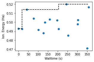
We can plot the training data against the time of simulation, showing that the model is finding better molecules over time.

train_data['time'] = train_data['time'] - train_data['time'].min()

fig, ax = plt.subplots(figsize=(4.5, 3.))

ax.scatter(train_data['time'], train_data['ie'])
ax.step(train_data['time'], train_data['ie'].cummax(), 'k--')

ax.set_xlabel('Walltime (s)')
ax.set_ylabel('Ion. Energy (Ha)')

fig.tight_layout()